Into Curve Invariant - part 1

The first part of this article is about the StableSwap invariant.

StableSwap

The Amplified Invariant is a mathematical concept introduced to improve the efficiency of liquidity pools by reducing slippage during trades while still allowing flexibility for price imbalance. It combines aspects of constant-sum and constant-product invariants to create a formula that balances between low slippage (near balance) and traceability at any price.

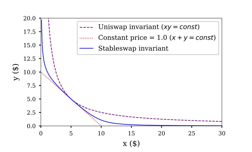
• Constant-product invariant (∏x_i=k): Used in Uniswap-like pools. It’s highly flexible and supports trades at any price, but slippage increases significantly for large trades.

• Constant-sum invariant (∑x_i=k): Used for stablecoins. It has no slippage for balanced trades but cannot handle large price imbalances.

• The Amplified Invariant combines the benefits of both: low slippage near balance and flexibility for imbalanced trades. The characteristic of the amplification coefficient parameter in StableSwap is that the lower it is, the closer the invariant is to the constant product.

A leverage factor χ is introduced to reduce slippage. This factor adjusts the shape of the invariant, allowing it to blend the properties of constant-product and constant-sum invariants, improving its efficiency across different trading scenarios.

The general formula is:

\(\chi D^{n-1} \sum x_i + \prod x_i = \chi D^n + \left( \frac{D}{n} \right)^n \space \space (1) \)

Where:

• χ: Leverage factor controlling the curvature of the invariant.

• D: Constant for the sum of token values at equilibrium.

• n: Number of tokens in the pool.

• ∑x_i: Sum of token amounts.

• ∏x_i​: Product of token amounts.

If this equation always holds, users will have trades with a leverage χ. However, it wouldn’t support prices going far from the ideal price 1.0. The invariant should support any prices (so that we have some liquidity at all times). So Stable Swap makes χ dynamic. When the portfolio is in a perfect balance, it’s equal to a constant A, however falls off to 0 when going out of balance:

\(\chi = \frac{A \prod x_i}{\left( \frac{D}{n} \right)^n} \space \space (2)\)

The StableSwap Invariant which adds χ into the general formula (1):

\(A n^n \sum x_i + D = A n^n D + \frac{D^{n+1}}{n^n \prod x_i} \space \space (3)\)

There are two frequent math operations to compute:

• Compute D given fixed values for A, and the reserves x_1,x_2,...x_n with n is the number of coins the pool supports, which is fixed when the pool is deployed.

• Given D, the user wishes to increase the value of one reserve xixi​ to x’_i and figures how much another reserve x_j​ needs to decrease to keep the equation balanced.

In Curve V1 (StableSwap), D behaves similarly to kk in Uniswap V2 - the larger D is, the more the reserves are, and the 'further out' the price curve will be. D changes and needs to be recomputed after liquidity is added or removed, or a fee changes the pool balance.

Calling S=∑x_i and P=∏x_i​, the equation (3) now is:

\(A n^n S + D = A n^n D + \frac{D^{n+1}}{n^n P} \space \space (4)\)

For example, if there are only two tokens in the pool, the invariant will become:

\(4AS + D = 4AD + \frac{D^3}{4P} \space \space (5) \)

In the StableSwap source code, it calculates D by calculating D_next:

The equation in this code can be written as:

\(D_{{next}} = \frac{(A n^n S + D_p n) D}{(A n^n - 1) D + (n + 1) D_p} \space \space (6)\)

For example, we have 100,000 USDC and 1,000,000 USDT in the pool. Using (3) or (4), we can calculate D approximately 1,094,540.84. This is a simple Python script for D with (5) (because it’s the example for (4)):

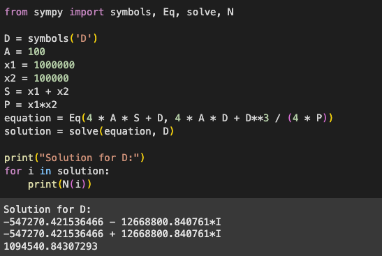
We could use that constant D again for calculating back amount of USDT or USDC by using (6).

StableSwap uses Newton's method to solve the equation numerically because it can not be solved algebraically. StableSwap creates f(D), equal to 0 when the equation (4) is balanced. In addition, it computes the derivative f′(D).

\((-A) n^n S - D + A n^n D + \frac{D^{n+1}}{n^n P} = f(D) \space \space (7) \)

\(\frac{(n+1)D^n}{n^n P} + An^n - 1 = f'(D) \space \space (8) \)

StableSwap solves for D using Newton's method, with D can be understood as the current value of D:

\(D_{next} = D - \frac{f(D)}{f'(D)} \space \space (9) \)

First, we can rewrite (8) by combining all elements into a single fraction and multiplying the top and bottom of the fraction by D, then :

\(f'(D) = \frac{\frac{(n + 1)D^{n+1}}{n^nP} + (An^n -1)D}{D} \space \space (10) \)

Rewrite the Newton's method by making the denominators equal f’(D), then substitute with (10):

\(D_{next} = \frac{D* f'(D) - f(D)}{f'(D)} \)

\(D_{next} = \frac{\frac{(n + 1)D^{n+1}}{n^nP} + (An^n -1)D - (-An^n S - D + A n^n D + \frac{D^{n+1}}{n^n P})}{\frac{\frac{(n + 1)D^{n+1}}{n^nP} + (An^n -1)D}{D}}\)

Distribute all the terms to remove the parenthesis in the numerator:

\(D_{next} = \frac{D(\frac{D^{n+1}}{n^nP} + \frac{nD^{n+1}}{n^nP}+ DAn^n -D + An^n S + D - A n^n D - \frac{D^{n+1}}{n^n P})}{\frac{(n + 1)D^{n+1}}{n^nP} + (An^n -1)D} \space \space (11)\)

After removing all of the cancellations in (11), we can define an element D_p as:

\(D_{p} =\frac{D^{n+1}}{n^n P} \)

The equation becomes:

\(D_{{next}} = \frac{(A n^n S + D_p n) D}{(A n^n - 1) D + (n + 1) D_p}\)

This equation is equal to the equation defined in (6).

Furthermore, in the Viper code, D_p is calculated by:

D_P: uint256 = D # D_P = S

for _x in xp:
    D_P = D_P * D / (_x * N_COINS)

xp is the number of tokens, so the loop will run n times. Therefore, we have D multiplied by itself n times in the denominator.

Then we can compute y or x’_j (the after value of x_j​) when a user increases the value of one reserve x_i​ to x’_i​.

With S=∑x_i and P=∏x_i. Assume to calculate token y with D, A, n; let's adjust the formula S and P a bit:

\( S = S' + y, \space P = P' * y\)

S′ and P′ are the sum and product of the balances of all tokens except the token y we want to calculate.

The formula then becomes from (4) to:

\(A n^n (S' + y) + D = A n^n D + \frac{D^{n+1}}{n^n P'y} \space \space (12)\)

Again, StableSwap uses Newton's method to solve the equation numerically. This time it creates f(y) and the derivative f′(y).

\((-A) n^n (S' + y) - D + A n^n D + \frac{D^{n+1}}{n^n P'y} = f(y) \space \space (13)\)

\(-(\frac{D^{n+1}}{n^n P' y^2} + An^n) = f'(y) \space \space (14)\)

StableSwap-Newton's method for y is:

\(y_{next} = y - \frac{f(y)}{f'(y)} \space \space (15)\)

Combine (13) and (14) for that equation, this can be transformed to:

\(y_{\text{next}} = y - \frac{-(A n^n (S' + y) + D - A n^n D - \frac{D^{n+1}}{n^n P'y})}{-(\frac{D^{n+1}}{n^n P' y^2} + An^n)} \space \space (16)\)

Again, rewrite the (16) method by making the denominators equal to (14):

\(y_{\text{next}} = \frac{y\frac{D^{n+1}}{n^n P' y^2} + yAn^n - A n^n (S' + y) - D + A n^n D + \frac{D^{n+1}}{n^n P'y}}{\frac{D^{n+1}}{n^n P' y^2} + An^n} \space \space (17)\)

On the other hand, (12) can be rewritten to f(ADn^n):

\( ADn^n = A n^n (S' + y) + D - \frac{D^{n+1}}{n^n P'y} \space \space (18)\)

Substituting into (17) then removing all cancellations:

\(y_{\text{next}} = \frac{y(\frac{D^{n+1}}{n^n P' y^2} + An^n)}{\frac{D^{n+1}}{n^n P' y^2} + An^n} \space \space (20)\)

We multiply the top and bottom by y/(A*n^n):

\(y_{\text{next}} *\frac{\frac{y}{An^n}}{\frac{y}{An^n}} = \frac{y^2(\frac{D^{n+1}}{n^n P' y^2} + 1)}{\frac{D^{n+1}}{n^n P' y An^n} + y} \space \space (21)\)

Rewrite the invariant (12) one more time into and substitute into (20):

\(\frac{D^{n+1}}{n^n P'y} = A n^n (S' + y) + D - ADn^n \space \space (22)\)

\(y_{\text{next}} = \frac{y^2(\frac{D^{n+1}}{n^n P' y^2} + 1)}{\frac{A n^n (S' + y) + D - ADn^n}{An^n} + y} \space \space (23) \)

The formula (23) can be performed as:

\(y_{\text{next}} = \frac{y^2 + \frac{D^{n+1}}{n^n P' A^n}}{S' + 2y + \frac{D}{A n^n} - D} \space \space(24) \)

In the Viper source, two variables are defined:

\(b = S' + \frac{D}{An^n} \)

\(c = \frac{D^{n+1}}{n^nP'An^n} \)

After substitution into the formula (24), we have:

\(y_{next} = \frac{y^2 + c}{2y + b - D} \)

There are two functions for y in the Curve source code, get_y and get_Y_D. The `get_Y_D` function calculates y from D, the same as the method above. In addition, `get_y` calculates new y when an amount of one token x changes from x to x'. Back to the example above, if we want to swap 10,000 USDT to get an amount of USDC, using the get_y function, the amount of USDC the user can get is 9,253.70. This is because, in the example, the amount of USDT is 10x of the USDC amount. So when the user swaps USDT into USDC, this causes slippage.

One point to note is the whitepaper of Curve uses invariant An^n (A * n ** n), but in the Viper source, the invariant is Ann (A * n * n).

The codebase instead computes A_ * n. This discrepancy arises because the codebase stores A_ as:

\(A\_ = An^{n-1}\)

Reference

https://docs.curve.fi/

https://www.rareskills.io/post/curve-get-d-get-y