Into Curve Invariant - part 2

The second part of this article is about the StableSwap invariant.

CryptoSwap

The CryptoSwap invariant is a core mathematical formula that defines the "liquidity curve" for Curve's trading pools, specifically designed for highly volatile asset pairs (not tightly pegged like stablecoins). It helps the pool concentrate liquidity around an "internal" price (determined through an internal oracle) and automatically adjusts when the pool becomes imbalanced. Here are the key points:

Combining advantages of two invariants:

• When the pool is balanced (value-equivalent balances), the CryptoSwap invariant behaves similarly to the stableswap invariant, creating a "flat" region (no slippage) that enables near 1:1 exchanges.

• When the pool becomes imbalanced, the invariant gradually shifts to constant-product invariant behavior (like Uniswap), resulting in increased slippage and protecting the pool against excessive price deviations.

Comparison of AMM invariants: constant-product (dashed line), stableswap (blue) and from this work (orange)

In Part 1, the StableSwap Invariant is described in the general formula:

\(\chi D^{n-1} \sum x_i + \prod x_i = \chi D^n + \left( \frac{D}{n} \right)^n \)

And the CryptoSwap invariant is encouraged by the StableSwap invariant:

\(KD^{n-1} \sum x_i + \prod x_i = KD^n + \left( \frac{D}{n} \right)^n\)

however, K is defined slightly differently:

\(K_0 = \frac{N^N \prod_{i=1}^{N} x_i}{D^N}, \quad K = A \cdot K_0 \cdot \frac{\gamma^2}{(\gamma + 1 - K_0)^2} \)

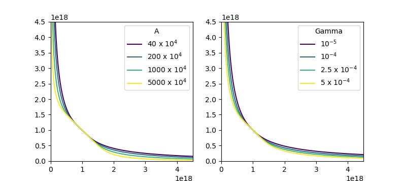
• A (amplification coefficient): The A parameter, similar to StableSwap invariant (Curve v1), controls how flat the bonding curve is at its center. This determines how concentrated liquidity is around the expected exchange rate (i.e., the "price scale"; see below)

• Gamma: The gamma parameter controls the separation between the two constant product curves shown in the above figure (dashed lines). When gamma increases, it stretches the "adjusted constant product" curve toward the lower-left corner, moving the curve's asymptotes closer to the axes and broadening the overall curve shape
  

Effects of adjusting the A (left) and gamma (right) parameters. For the left plot, gamma = 0.000145. For the right plot, A = 400,000.

The init:

\(D_0 = N \left( \prod x_k \right)^{\frac{1}{N}} \)

With the initial formula, we can rewrite f(D_0) as in a situation which only has 2 coins:

\(D_0 = \sqrt{x[0]x[1]} <=> D_0^2 = x[0][1] \)

\(f(D_0) = D_0^2 -x[0]x[1] \)

\(f'(D_0) = 2D_0 \)

Using Newton's method, the Initial values can be transformed to:

\(D_{0_\text{next}} = D_0 - \frac{f(D_0)}{f'(D_0)} \)

\(D_{0_\text{next}} = D_0 - \frac{D_0^2 -x[0]x[1]}{2D_0} \)

\(D_{0_\text{next}} = \frac{D_0 - \frac{x[0]x[1]}{D_0}}{2} \)

With this formula, D_0 can be calculated by looping through A time. In the viper code, A is set to 255.

The code calculates the absolute difference between the current and previous values of D_0. It stops iterating when the difference is either very small (diff ≤ 1) or when the difference multiplied by 10^18 is less than D_0. Once one of these conditions is met, the function returns the converged value of D_0.

Back to the invariant, let S be the sum of x_i and P is the product of x_i. f(D) with 2 coins (N = 2) becomes:

\(K_0 =\frac{4D}{D^2}, K = A \cdot K_0 \cdot \frac{\gamma^2}{(\gamma + 1 - K_0)^2} \)

\(f(D) = KDS + P - KD^2 - \frac{D^2}{4}. \)

The derivative of f(D) is:

\(f'(D) = K'\cdot D(S - D) + K(S-2D) - \frac{D}{2} \)

This can be transformed to:

\(f'(D) = -2\gamma^2 AK_0 \frac{(\gamma +1 + K_0)}{(\gamma +1 - K_0)^3}(S-D) + AK_0\frac{\gamma^2}{(\gamma +1 - K_0)^2}(S-2D) - \frac{D}{2} \)

The above formula can be transformed to simplify. First, divide all terms by K and expand everything inside the parentheses.

\(f'(D) = \frac{-2\gamma^2 AK_0 \frac{(\gamma +1 + K_0)}{(\gamma +1 - K_0)^3}(S-D)}{K} + \frac{AK_0\frac{\gamma^2}{(\gamma +1 - K_0)^2}(S-2D)}{K} - \frac{D}{2K} \)

\(f'(D) = \frac{-2\gamma^2 AK_0 \frac{(\gamma +1 + K_0)}{(\gamma +1 - K_0)^3}(S-D)}{ A \cdot K_0 \cdot \frac{\gamma^2}{(\gamma + 1 - K_0)^2}} + \frac{AK_0\frac{\gamma^2}{(\gamma +1 - K_0)^2}(S-2D)}{A \cdot K_0 \cdot \frac{\gamma^2}{(\gamma + 1 - K_0)^2}} - \frac{D}{2 \cdot A \cdot K_0 \cdot \frac{\gamma^2}{(\gamma + 1 - K_0)^2}} \)

\(f'(D) = -2\frac{\gamma +1 + K_0}{\gamma +1 - K_0}(S-D) + S - 2D - \frac{D(\gamma + 1 - K_0)^2}{2AK_0\gamma^2} \)

\(f'(D) = -2\frac{\gamma +1 + K_0}{\gamma +1 - K_0}S + 2\frac{\gamma +1 + K_0}{\gamma +1 - K_0}D + S - 2D - \frac{D(\gamma + 1 - K_0)^2}{2AK_0\gamma^2} \)

Now S can be written as - S + 2S:

\(f'(D) = -2\frac{\gamma +1 + K_0}{\gamma +1 - K_0}S + 2\frac{\gamma +1 + K_0}{\gamma +1 - K_0}D - S + 2S - 2D - \frac{D(\gamma + 1 - K_0)^2}{2AK_0\gamma^2} \)

Then, factor out the common terms between the groups containing S and D.

\(f'(D) = -2S(\frac{\gamma +1 + K_0}{\gamma +1 - K_0} - 1) + 2D(\frac{\gamma +1 + K_0}{\gamma +1 - K_0} - 1) - S - \frac{D(\gamma + 1 - K_0)^2}{2AK_0\gamma^2} \)

Make all denominators inside the parentheses common:

\(f'(D) = -2S(\frac{\gamma +1 + K_0 - \gamma -1 + K_0}{\gamma +1 - K_0}) + 2D(\frac{\gamma +1 + K_0 - \gamma -1 + K_0}{\gamma +1 - K_0}) - S - \frac{D(\gamma + 1 - K_0)^2}{2AK_0\gamma^2} \)

\(f'(D) = -2S(\frac{2K_0}{\gamma +1 - K_0}) + 2D(\frac{2K_0}{\gamma +1 - K_0}) - S - \frac{D(\gamma + 1 - K_0)^2}{2AK_0\gamma^2} \)

\(f'(D) = -\frac{4SK_0}{\gamma +1 - K_0} + \frac{4DK_0}{\gamma +1 - K_0} - S - \frac{D(\gamma + 1 - K_0)^2}{2AK_0\gamma^2} \)

Introduce two auxiliary variables, mul1 and mul2, to simplify the variables in the function:

\(\text{mul1} = \frac{D(y + 1 - K_0)^2}{4Ay^2} \)

\(\text{mul2} = \frac{4K_0}{y + 1 - K_0} \)

The derivative f'(D) now can be reduced to:

\(f'(D) = - S - S\cdot\text{mul2} - \frac{2\text{mul1}}{K_0} + D\cdot\text{mul2} \)

In the viper code, _g1k0 variable is defined to be:

\(\text{_g1k0} = \gamma + 1 - K_0\)

Back into the code,

This code calculates -f'(D) instead of f'(D). This makes Newton's step more clear. In addition, f(D) is divided by K:

\(f(D) = DS + \frac{P}{K} - D^2 - \frac{D^2}{4K} \)

\(f(D) = DS + \frac{D^2K_0(\gamma + 1 -K_0)^2}{4AK_0\gamma^2} - D^2 - \frac{D^2}{4K} \)

\(f(D) = DS + \frac{D^2(\gamma + 1 -K_0)^2}{4A\gamma^2} - D^2 - \frac{D^2(\gamma + 1 - K_0)^2}{4AK_0\gamma^2} \)

\(f(D) = DS - D^2 - \frac{D^2(\gamma + 1 - K_0)^2}{4A\gamma^2}(\frac{1}{K_0} - 1) \)

\(f(D) = DS - D^2 - D\cdot\text{mul1}(\frac{1}{K_0} - 1) \)

The full Newton's method for D now is:

\(D_{next} = D - \frac{f(D)}{f'(D)} = \frac{D(-f'(D)) + f(D)}{-f'(D)} \)

The formula has been separated into two parts for Newton's method:

\(D_{\text{plus}} = \frac{D(-f'(D)) + DS}{-f'(D)} \)

\(D_{\text{minus}} = \frac{D^2 + D\cdot\text{mul1}(\frac{1}{K_0} - 1)}{-f'(D)} \)

The final D will be calculated as the difference between the two equations above.